- Research
- Open access
- Published:
Quantitative coating thickness determination using a coefficient-independent hyperspectral scattering model
Journal of the European Optical Society-Rapid Publications volume 13, Article number: 40 (2017)
Abstract
Background
Hyperspectral imaging is a technique that enables the mapping of spectral signatures across a surface. It is most commonly used for surface chemical mapping in fields as diverse as satellite remote sensing, biomedical imaging and heritage science. Existing models, such as the Kubelka-Munk theory and the Lambert-Beer law also relate layer thickness with absorption, and in the case of the Kubelka-Munk theory scattering, however they are not able to fully describe the complex behavior of the light-layer interaction.
Methods
This paper describes a new approach for hyperspectral imaging, the mapping of coating surface thickness using a coefficient-independent scattering model. The approach taken in this paper is to model the absorption and scattering behavior using a developed coefficient-independent model, calibrated using reference sample thickness measurements performed with optical coherence tomography.
Results
The results show that this new model, by considering the spectral variation that can be recorded by the hyperspectral imaging camera, is able to measure coatings of 250 μm thickness with an accuracy of 11 μm in a fast and repeatable way.
Conclusions
The new coefficient-independent scattering model presented can successfully measure the thickness of coatings from hyperspectral imaging data.
Background
Non-destructive evaluation and metrology of engineering and natural materials are of interest and a challenge in many industry sectors, including engineering, manufacturing, biomedical, cultural heritage and research. In the paints and coatings industry, layers of paints and coatings, with a typical thickness in the range of micrometers to millimeters, are applied to substrates of different materials. In some cases, multiple layers are applied either with different material properties, or to facilitate the drying process when applying a thick coating. It is of interest both directly after application and for in-situ assessment of cracks and delaminations to measure the coating layer thickness, to confirm the application procedure and to decide when repainting is needed.
Techniques for structural and thickness measurements of paints and coatings can be classified as point measurement or field measurement. Point measurement techniques include destructive sampling and inspection under a microscope, ultrasonic techniques based on pulse-echo ultrasonics [1], spectroscopic ellipsometry and low-coherence interferometry [2]. Field measurement techniques include digital holographic techniques [3], spectral reflectance optical coherence tomography [4, 5] and other scanning probe setups. The point measurement techniques provide limited spatial information and the field techniques are typically slow and introduce challenges in scanning and automation.
Hyperspectral imaging is a remote-sensing technique used to obtain spectral reflectance information about materials from large scale surface areas of square-kilometers to small surfaces of square-millimeter area [6]. It is used in multiple application fields, including medicine [7,8,9], remote sensing [10], agriculture [11], engineering [12] and cultural heritage [6, 13]. Although the range of research fields in which hyperspectral imaging has been applied is vast, the existence of a quantitative hyperspectral imaging approach able to provide thickness information of thin layers could offer new applications beyond the aforementioned fields [14].
In this work we propose a new method of thickness measurement for semi-transparent coatings, based on hyperspectral imaging. Initially we investigated the existing absorption model of Lambert-Beer (LB) and the absorption-scattering model of Kubelka-Munk (KM). Further investigation of the spectral properties of the coating led to the development of the coefficient-independent (CI) approach presented in this paper, which we have benchmarked against the LB and KM models experimentally.
Theory
This theory section, first describes the theory of hyperspectral imaging, then presents the Lambert-Beer and Kubelka-Munk models. It then describes the theory of our new coefficient-independent approach.
Hyperspectral imaging
Hyperspectral imaging (HSI) is an optical technique that is mostly used to obtain compositional information about the surface of a sample [6]. In its most simple form, this technique records the light spectrum from a beam reflected from or scattered by a sample using a spectrometer [15], across a surface by using a two-dimensional spatial scanner. Since the recorded reflectance and scattering information of light at a certain frequency can be related to a specific energy level and structure of the surface, measurements have the potential to provide very precise information about the sample’s surface composition. Based on the sensor used, the frequency range for this measurement can vary between the ultraviolet and the infrared range, with the visible and near infrared light (400-1000 nm) to be mostly used due to the good availability of silicon based sensors.
Other approaches use scanning in the spectral domain by using interference filters mounted on filter wheels [16]. Based on the latest advances, hyperspectral imaging is performed in one full spatial and one full spectral dimension (line spectral imaging). The generation of the 3D dataset (called a spectral cube) is achieved by sample movement along a scanning platform, which is responsible for the second spatial dimension (Imspector from Specim, Linescan from imec). As a result, the acquired spectral cube contains a full spectrum at each image pixel, that, just like in reflectance spectroscopy, can be related to the sample’s surface material composition.
Being a combination of reflectance spectroscopy with digital imaging, hyperspectral imaging contains advantages from both the spectroscopic (i.e. the non-contact optical non-destructive testing), and the digital imaging point of view (the various scales of field of view). The most unique advantage of this technique is the ability to map quantitatively selected wavelength features on the examined field of view.
Lambert-beer model
The Lambert-Beer (LB) law is an empirical law for the attenuation of light, due to absorption and scattering, reaching the detector, over a specified optical path length. The Kubelka-Munk model, described below, includes additional scattering terms, but reduces to the LB law when the scattering coefficient goes to zero [17]. The sample can be visualized as a two-layered structure, namely a substrate with a coating on top, where the main contribution to the measured reflectance is due to diffuse reflection at the substrate-coating boundary, but is decreased by attenuation within the coating on top of the substrate, both before and after reaching the coating-substrate boundary. This model will be referred to as the LB model and is shown schematically in Fig. 1.

The LB model assumes incoming light is diffusely scattered by the substrate (1), after which absorption (2) and further scattering (3) decreases the amount of reflected light recorded by the detector
When performing an hyperspectral imaging scan, the measured reflectance \( {\mathrm{R}}_{\uplambda_{\mathrm{i}}} \) at a certain wavelength was approximated based on the LB law by:
where the measured intensity at wavelength λi is seen as a multiplication of the reflectance of the light diffusely scattered from the substrate-coating boundary at that specific wavelength, \( {\mathrm{R}}_{\mathrm{s},{\uplambda}_{\mathrm{i}}} \) and an exponential term taking into account the loss of reflectance due to attenuation in the coating. The amount of absorption per wavelength band is dependent on the path that the light travels, δ, and what will be referred to as the extinction coefficient \( {\mathrm{k}}_{\uplambda_{\mathrm{i}}} \) [17]. Due to the geometry of the setup with illumination at a 45° angle, δ is equal to (1 + √2) times the geometrical thickness d of the coating layer.
When the extinction coefficient is known, a reference spectrum of the substrate underneath the coating can be used to find the thickness of the layer as a function of wavelength:
An easy way to determine the extinction coefficient for a specific coating is by inverting Eq. (1) and using a known thickness in combination with a known substrate reflectance spectrum. The thickness can, for example, be determined using an Optical Coherence Tomography (OCT) depth scan [18]. OCT is a technique based on low-coherence interferometry to measure light reflections from refractive index interfaces and is a suitable technique for imaging the interfaces in a semi-transparent material and therefore for measuring coating thickness.
Kubelka-Munk model
One of the most widely used models to describe the optical properties of paint and coating layers, is the Kubelka-Munk (KM) model. This model is also known as the two-flux radiative transfer model, referring to the light fluxes traveling upwards and downwards in the coating layer [19]. In this model, absorption and scattering are incorporated as two independent coefficients K and S. The diffuse reflectance \( {\mathrm{R}}_{\uplambda_{\mathrm{i}}} \) at wavelength λi is related to K and S coefficients and the thickness of the layer, d, through:
where \( {R}_{s,{\lambda}_i} \) is the diffuse reflectance from the substrate, a = (S + K)/S and b = (a2–1)1/2 for the wavelength λi. Even though the KM model is frequently used in hyperspectral imaging [20], the applicability of the theory has been questioned by some [21]. The main reason for questioning the applicability of the KM model to a coating on a substrate is because originally, reflectance in the KM model was measured using an integrating sphere, rather than a spectrometer collecting light through an objective lens.
A possible way to determine the K and S coefficients of a certain coating and for all wavelengths is by applying the coating to two different substrates with known reflectances and thicknesses and solving Eq. (3) twice for the two unknown K and S. Once these coefficients are known, they can be used to determine the thickness of any layer of which the substrate reflectance is known, as will be shown in the results section.
Coefficient-independent approach
In order to reach the objective of this paper and perform large scale coating thickness measurements using hyperspectral imaging, a new coefficient-independent model has been developed. A CI model has benefits over the KM and LB models, which results in shorter measurement procedures and better fitting to experimental data, rather than the calculation of different coefficients. Secondly, this coefficient-independent model fully uses the abundance of spectral information rather than calculating the thickness from the reflectance at a single wavelength. This model was used to address the research objectives shown in Fig. 2.

When combining OCT and hyperspectral imaging, theoretical models can be calibrated in order to calculate the thickness of a coating in a larger area
The novel CI model does not consider any material optical coefficients and is aimed at linking the unique spectral characteristics of reflected light to coating thickness. Such characteristics can be established for any coating and assuming partial transparency at some wavelengths measured, should be able to measure the coating thickness after calibration. Examples of such behavioral characteristics are: the wavelength where a certain thickness coating becomes transparent, the wavelength where a certain thickness coating does not fully absorb the incoming light anymore, and the rate of change in absorbance over a certain wavelength range. These characteristics are shown in Fig. 3, where the slope in a certain wavelength range is shown to be thickness dependent. This model will be referred to as the coefficient-independent model and the data-processing results of this model will be compared with the LB and KM models.

The spectrum from a thicker layer of coating becomes transparent at a different wavelength and reaches a different maximum reflectance. These characteristics, and most specifically the slope in a certain wavelength range, can be used to link a spectrum to its corresponding coating thickness
For any semi-transparent coating, an empirical linear relation can be established between coating thickness and the slope of the reflectance in a particular wavelength range. Again, the influence of the combined scattering and absorption can be assumed to be exponential and the measured reflectance R to depend on substrate reflectance RS and on a function α(λ):
which would make the derivative with respect to wavelength:
If RS is constant for small wavelength ranges and the exponential approaches 1, meaning that the absorption is low, it can be seen that \( \frac{\mathrm{d}\mathrm{R}}{\mathrm{d}\uplambda \kern0.5em } \) is directly dependent on the distance that the light travels in the material, namely δ.
Experimental setup
Hyperspectral imaging
The hysperspectral imaging setup used in this study consisted of an IMSPECTOR V10E (Specim©) spectral camera, operating in the 400–1000 nm range. It has a camera with 1312 by 1082 pixels and a frame rate of 108 fps. The optical bandwidth is 2.73 nm. The visible range was selected due to the main absorption characteristics of the studied coating layers which is within the range of 400-1000 nm.
The setup is shown in Fig. 4. Samples were scanned with a Specim Labscanner automated scanning platform, which can scan an area of 200 by 65 mm in 1 s. The spatial resolution achieved is 0.2 by 0.6 mm. The geometry of the setup was such that the recording of specular reflections was minimized, by placing the light source under a 45-degree angle with respect to the surface plane. Adjusting the lens of the system changed the total length of one 2D measurement; the speed of the scanning platform, the frame rate and the number of frames acquired defined the total size of the scanned area. Only the 450–950 nm range provided results with a good signal to noise ratio (SNR) and this range will therefore be used in this research.

Hyperspectral imaging is used to obtain spectral information at every x-y position. This spectral information contains chemical information about a material due to the unique interaction between the light and the material
Post-processing of hyperspectral imaging data involved normalization at every wavelength using a white reference image acquired from a diffuse Spectralon reflectance target (SRT-MS-050, Laser2000) and a dark reference image obtained with a closed shutter. The dark reference image was first subtracted from both the white reference and the actual measurement at each wavelength in order to correct for thermal dark current [6]. Next, the resulting data set was divided by the white reference in order to correct for illumination and gain variations across the detector and to obtain the reflectance. The final data processing step was aimed at linking spectral information to the thickness of the coating layer. For this purpose, three different theoretical models were tested and will be discussed in a later section.
OCT system for thickness calibration
As shown in Fig. 5, a customized OCT system was built by using a superluminescent diode (FESL-1550-20-BTF, Frankfurt Laser Company) centered at 1550 nm with a full width at half maximum of 60 nm, resulting in an 11 μm theoretical axial resolution inside the coating layer (considering a refractive index of 1.5). The spot size is 20 μm diameter. Depth-scanning for OCT was realized by the means of an optical delay line (ODL-650,MC, OZ Optics, Ltd). Lateral scanning of a sample with an x-y translation stage (T-LS28M, Zaber Inc., Canada) allowed for a 28 mm scanning range in two directions. Obtained data were bandpass filtered and an envelope detector was used to recover the depth dependent signal [22].

Schematic design of OCT based on a Michelson interferometer
Sample preparation
In order to test the coefficient-independent model as well as compare it to the existing KM and LB models, samples of a coating on different substrates were prepared. The coating selected in this research was a film-forming low-gloss wood lacquer for outdoors (Transparant zijdeglanslak voor buiten, Wijzonol Bouwverven B.V.). This coating was selected because it is semi-transparent and is a commonly used wood coating, making it a suitable coating to visualize with OCT and hyperspectral imaging. This spruce-colored coating is based on organic solvent with an alkyd binder and applied using a brush. The samples that were prepared are:
-
1)
Coating on a very flat and reflective silicon wafer to be able to determine the refractive index of the coating.
-
2)
Different thickness coatings applied to thin cover glasses in order to be able to determine the K and S coefficients from the KM-model and the extinction coefficient from the LB model. In order to measure the coefficients, these cover glasses were placed on a black-and-white checkerboard, as described below.
-
3)
One to four layers of the coating were applied to a Medium-Density Fibreboard (MDF) plate covered with acrylic gesso. This reflective non-absorbing background serves as a reference for assessing the performance of the models.
It should be noted that the aim of this paper is to show the general feasibility of the proposed model rather than the applicability to a specific coating. Based on our model, pigmented and less transparent coatings can also be measured, as long as they become transparent within the wavelength sensitivity range of the sensor. For the scope of this paper, we only focused on the analysis on the aforementioned samples.
Methods
Calibration and measurement procedure
The calibration procedure was used to establish the model coefficients for the LB, KM and CI models. The main steps of the calibration procedure are described below (a-f):
-
Step (a):
Determine the refractive index of the coating by measuring the optical thickness of a coating reference of known thickness with OCT. Determining optical thicknesses of coating layer from an OCT linescan can be done in a straight-forward way by comparing the optical distance between the first and second reflection peaks. These peaks can be located by using Gaussian fitting, considering the Gaussian light source used in the OCT system. The refractive index is then determined from the ratio of the optical thickness and physical thickness of the coating. This physical thickness can be determined in multiple ways, for example from a cross-sectional OCT profile scan, as shown later in Fig. 6a.
Fig. 6 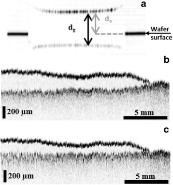
a) By determining the optical and geometrical thickness (do and dg) using OCT on a strip of coating on silicon wafer, its refractive index n can be determined. The optical thickness is 700 μm for a 1.5 cm linescan. An OCT linescan (b) of partially coated gesso shows that the difference in refractive index between coating and air disturbs the image. By correcting for the refractive index (c), the geometrical thickness can be plotted
-
Step (b):
Perform a thickness profile of a coating reference sample of varying coating thickness using OCT. By translating the scanning probe laterally and scanning a depth line at each lateral location, a cross-sectional profile can be acquired. In the same way as indicated in step (a), the optical thickness of a coating at different locations can be measured and thus converted into a geometrical thickness using the calculated coating refractive index. This geometrical thickness profile can then be used as a reference for calculating the coefficients for each model.
-
Step (c):
Perform a hyperspectral imaging scan of the coating reference sample with varying coating thickness in order to confirm the roles of both scattering and absorption in the light-matter interaction. Samples are placed on the scanning platform of the hyperspectral imaging system, which is optimized based on the selected field of view and focused. The scanning stage parameters are set based on the scanning speed (mm/s) and the maximum number of line scans to be acquired. If the obtained spectra show influence from both scattering and absorption in the coating, the theory on the KM and LB models can be applied.
-
Step (d):
Calculate the LB parameters \( {\mathrm{R}}_{\mathrm{s},{\uplambda}_{\mathrm{i}}} \) and kλ for each hyperspectral wavelength. In order to be able to assess the results generated with the coefficient-independent model, a comparison with the known KM and LB models will be made, for which a calculation of the different coefficients is required. The required coefficients for the LB model can be calculated as described in the theoretical section. The thickness of the coating layers for these calculations is provided by OCT as described in (b). Since there are no reference coefficients available for any of the models and coatings, assessing the validity of the obtained coefficients was based on pre-determined criteria. First of all, the differences in the coefficients obtained from different thickness layers should be small, namely in the range of uncertainty in the calculations of these thicknesses. Secondly, even though the thickness can be calculated from the spectrum at any wavelength band, they should all result in the same value. By inverting Eq. (1) and Eq. (2) from sections 2.3 and 2.4 respectively, the extinction coefficient as well as the K and S coefficients can be found.
-
Step (e):
Calculate the KM parameters \( {\mathrm{R}}_{\mathrm{s},{\uplambda}_{\mathrm{i}}} \), Sλ and Kλ for each hyperspectral wavelength. In order to calculate the KM model coefficients, the known thickness coating-on-glass samples were placed on a black-and-white checkerboard sheet. The reflectance of the white background with coating and glass was compared with the reflectance of white covered with glass without coating. The same procedure was repeated for the black background, as described in section 2.3. This process was repeated twice for different thickness layers in order to validate the obtained coefficients.
-
Step (f):
Calculate the CI parameters \( {\mathrm{R}}_{\mathrm{s},{\uplambda}_{\mathrm{i}}} \) and \( {\mathrm{dR}}_{\mathrm{s},{\uplambda}_{\mathrm{i}}}/ d\lambda \) for each hyperspectral wavelength. The aim of the coefficient-independent model is to find the thickness of a coating layer without determining coating-specific coefficients but rather to make use of the spectral characteristics of different coating thickness layers.
The calibration steps will be followed by a comparison of the different models by comparing the thickness profile of a sample calculated with the different models to an OCT linescan.

Results and discussion
Performance of the calibration procedure
In step (a), the refractive index of the coating was determined as 1.506 ± 0.014 at 1550 nm, which is an error of around 1%. This error is acquired by statistical analysis of the refractive indices measured at different locations on the coating. This error is consistent with the error in peak detection. That is half of the sampling interval in a depth scan, which is 4.8 μm or roughly 1% of the geometrical thickness of the coating.
Step (b). Figure 6 shows a linescan of a layer of coating on spruce, without correction for the refractive index of the coating (Fig. 6b) and with correction (Fig. 6c). From the corrected data, a thickness profile can be determined at the line where the scan was made, and the thickness at a single point can be extracted. This shows the thickness varies between 0 and about 400 μm.
Step (c). Hyperspectral imaging measurements show that both scattering and absorption play a role in the interaction between light and coating, as was the assumption at the basis of two of the theoretical models. Figure 7b shows different obtained spectra for the spruce-colored coating with the reference black and white substrate spectra measured on the sample shown in Fig. 7a. The spectrum of the coating on the white substrate is shown for two different thickness coating layers, namely 240 and 170 μm coating layers respectively. The small peak around 620 nm is consistent with noise from the standard fluorescent light sources in the lab.

The KM and LB model coefficients are measured using a strip of coating on glass, placed on a black-and-white checkerboard background (a). Five spectra at different backgrounds and thicknesses (b) show the influence of scattering, absorption and coating
In the 450–580 nm range, the spectra of the coating on both black and white backgrounds seem to be very similar. In this range, the measured intensity is even lower than the measured intensity of the black background, meaning that the light most likely does not even reach the background at this point and almost all of the light is absorbed in the coating layer. Above 580 nm, the background does seem to have an influence on the measured back-reflected intensity, as the spectra from the black and white backgrounds are different. The intensity recorded from the coating on a white background is clearly lower than the reflectance from the background only. This indicates absorption and possibly scattering of light away from the detector.
Also, for the coating on the black background between 600 and 900 nm, the recorded intensity is higher than the background reflectance. This could be due to scattering of light in the coating, in the direction of the detector. Lastly, it can be seen that the maximum reflectance of the recorded spectrum from the coating on the white background is decreasing with coating thickness. The influence of absorption and scattering on reflectance is thus a function of thickness. In conclusion, absorption and scattering do seem to play an important role in the light-coating interaction and their influence varies with wavelength and thickness.
Steps (d) and (e): see Fig. 8a and b. The wavelengths from 450 to 600 nm are not suitable for use by either model. In the case of the LB model in Fig. 8a, different thickness coating layers in this region amount to different calculated extinction coefficients; therefore, applying each extinction coefficient to an obtained hyperspectral imaging spectrum will result in different obtained thicknesses. In addition to that, the KM model coefficients could not be solved in that same spectral range, as seen in Fig. 8b. For both models, this is probably because there is very high absorption in this region; the exponential function will turn reflectances tending to zero into LB model coefficients going to infinity and the solutions when solving for the K and S coefficients of the KM model will not be stable.

The extinction coefficient (a) calculated from the LB model is not the same when calculated for different thickness samples in the 450–600 nm range, therefore this part of the spectrum is not useful when calculating the thickness from the LB model. The K and S coefficients (b) from 600 to 950 nm are very similar when calculated from different thickness layers
In both models, different thickness coating layers lead to slightly different obtained coefficient values, with differences in the order of 1.3% (K coefficient), 6.7% (S coefficient) and 6.0% (extinction coefficient).
These differences could still be explained by wrongful determination of either one or both of the thicknesses of 2% on top of a 6% error of linking the thickness information from the OCT line scan to the hyperspectral imaging 2D image. However, this 6% error is not an error of the technique. This error can be reduced when either the special variation of thickness of the coating layer is reduced or by improving the accuracy of the spatial correlation between the OCT and HSI data from its current value of ±0.5 mm.
Step (f). When plotting the spectra of different thickness layers, it can be seen in Fig. 9a that the wavelength, at which the reflectance of a particular thickness layer starts to increase significantly, is thickness-dependent. This is most likely related to the relationship between wavelength and the penetration of light into the coating layer. Shorter wavelengths penetrate less deeply into the coating layer, while longer wavelengths reach deeper. In the case of thin layers, shorter wavelengths can reach through the coating layer to the reflective substrate, while for thicker layers this can only happen at longer wavelengths.

(a) Five obtained spectra for different thickness layers show that the thickness is a determining factor for measured reflectance. The slopes of these spectra (b) show that in the 500–650 nm range, both the maximum slope and its corresponding wavelength are thickness dependent
As a result of the difference in wavelength at which the coating becomes partially transparent as well as the difference in maximum reflectance, the slope of a spectrum is a good starting point for the coefficient-independent model. A plot of the slope of all spectra, as shown in Fig. 9b, confirms that both the maximum value of the slope as well as the wavelength at which this maximum slope value occurs, is different for different coating thicknesses. This is most likely related to the concept described in section 3.1, namely that the derivative of an exponential function depending on the thickness has a linear relationship locally with the thickness. Especially the 560–580 nm wavelength range is suitable for linking slope to thickness. Figure 10 shows the linearity when the thickness is plotted against the average slope in the 560-580 nm wavelength range (Fig. 10a), against the wavelength band where the maximum slope occurs (Fig. 10b) and the value of the slope at that maximum (Fig. 10c). By performing the same steps on any spectrum, the linear trendline can relate slope, maximum slope or wavelength at maximum slope to coating thickness. It can be seen from Fig. 10a that the maximum thickness that can be measured in this way, will not exceed 230 μm. Dividing the maximum slope value by the wavelength range at which this maximum occurs, may increase the upper limit to a thickness determination to more than 250 μm, as seen in Fig. 10d. Theoretically, the minimum thickness that can be measured in this way is related to the axial resolution of the OCT setup, 11 μm. The actual resolution is difficult to estimate.

Linear relations can be found between thickness and certain spectrum characteristics. This holds for thickness plotted against average slope in the 560–580 nm range (a), against the wavelength where a peak in slope occurs (b) and the value of this peak in slope (c). In order to extend the dynamic range of thickness measurement, plots b and c can be divided to obtain (d), where the maximum thickness that can be measured is larger than 250 μm
The linear relationships shown in Fig. 10 can be used to determine the thickness of a coating layer in a centimeter-by-centimeter area. When the same characteristic are determined for any spectrum as the characteristics used to create the plots in Fig. 10, the resulting value can be linked to a corresponding thickness using the linear trend line.
This is shown in Fig. 11. The method provides results for two different linear relations, namely the relationship between thickness and slope in the 560–580 nm range and ratio between the maximum of the slope and the wavelength at that maximum slope. In this way, a thickness plot is made of a coated area.

Two regions in (a) are used to test the success of using the average slope in the 560–580 nm range (b and d) and the ratio between maximum slope value and the wavelength at this maximum (c and e). All thickness maps are very similar, but the map created from the maximum slope divided by the wavelength at this maximum is coarser. The thickness of all plots is given in μm
Comparison of results of KM and LB models
In order to be able to assess the results generated with the coefficient-independent model, a comparison with the known KM and LB models will be made. As shown in the previous section, modeling the thickness of a layer of coating using the obtained coefficients shows that both the KM and LB models succeed in finding realistic and similar coating thicknesses, but only at certain wavelengths. A first step in assessing the validity of the obtained outcomes is therefore whether different wavelength components give similar results. This was done at the 600–950 nm range as the 450–600 nm had proven to be unsuitable in section 4.3. Figure 12 shows the calculated thicknesses of a thick and a thin coating area of coating using both models.

When calculating the thickness of a thick and thin coating layer for different wavelengths, this calculated thickness differs by a maximum of 23.3 μm for the LB model and 40.6 μm for the KM model for different wavelengths
The LB model produces results that vary by 23.3 μm in thickness for the thick layer between 600 nm and 950 nm and 11.3 μm for the thin layer, so 9.6% and 14.4% of the mean thicknesses respectively. In the case of the KM model, the variation is slightly larger, namely increases of 40.6 μm and 19.9 μm for the thick and thin layers, 17.3% and 28.5% percent of the mean thickness respectively.
Wavelength-dependent variations in the calculated thickness may be expected because both models make a number of simplifications. First of all, losses in reflectance between uncoated and coating substrate due to the specular reflections from the air-coating interface are ignored. Since the refractive index of the coating layer is wavelength dependent, this may induce a wavelength-dependent error. Secondly, since the air-coating interface is not perfectly flat, a wavelength-dependent scattering from this interface may scatter more or less incoming light in the direction of the detector. Improving this could be done by adding a certain percentage of the specular reflection into account, depending on the surface roughness. Either way, these results show that the hyperspectral-nature of the dataset becomes a disadvantage rather than an asset in the KM and LB models.
Accuracy of the coating thickness measurement using the LB, KM and CI methods
In order to be able to check whether one of the models is able to obtain the “true” coating thickness, the calculated thicknesses are compared with the geometrical thickness at that point calculated from the optical thickness obtained with OCT. At a single line in a hyperspectral imaging dataset, the different models combining hyperspectral imaging with OCT were applied. An OCT linescan was performed at the same location, see Fig. 13.

When comparing the different models to the OCT reference measurement, the coefficient-independent model is most successful. The LB and KM models are not very accurate
It can be seen that the coating-independent model in the two configurations also shown in Fig. 13 is most successful in finding coating thickness values close to that OCT reference value than the KM and LB models. The fact that no calculation of coefficients is needed makes this technique easier to implement and adapt to any coating based on coating-specific spectral features. A calibration is still required, but this calibration can be done without preparing an additional sample.
Discussion
The results from the KM model show that it may not be the best model for determining coating thickness for this particular coating. The obtained thickness is not wavelength-independent and also not as close to the real thickness as the coating-independent model. A possible explanation may be the fact that the original KM calculations were performed with a setup with an integrating sphere rather than a hyperspectral imaging setup as used in this research. In addition to that, the spectra of the coating show that absorption plays a larger role than scattering, while scattering media will result in more diffuse illumination, therefore better meeting the original conditions under which the model was developed. Lastly, the need to prepare separate samples with coating on glass excludes unknown or new coatings already applied to a substrate and induces the possibility for additional errors as well as results in extra computation and measurement time. Reference thickness measurements still need to be performed for the new coefficient-independent model, but these can be done locally using OCT, after which a thickness in a large area can be determined. Other adaptations of the KM model have been proposed in literature but not all of these have been tested. The most general KM model has been used and described here and a comparison with the other versions is beyond the scope of this paper.
The LB model is less wavelength-dependent than the KM model, but the agreement with the thicknesses measurements made with OCT is worse than the KM model. This may be a result of the simplification adopted in the model, namely that scattering only results in less light reaching the detector rather than more. The LB model also requires a calibration measurement under the condition that the substrate material for calibration is sufficiently scattering rather than absorbing the incoming light. This may offer an advantage with respect to the KM model: if the substrate material of the sample under investigation is sufficiently scattering, there is no need to prepare reference samples on glass to calculate the extinction coefficient. A last problem with the LB model is that it was originally developed for measuring light transmitted through a material. In this case, the light is assumed to travel through a coating layer twice after it is scattered from a substrate, which is a much more complicated situation that may not be modeled in such a simplified way as shown in Fig. 1.
Hyperspectral imaging is also a promising technique for monitoring coating quality over a period of ageing, as changes in spectral characteristics may be early indicators of damages to a coating or the substrate underneath. An additional advantage of using a coating-independent model during an ageing process is that such a model will not be affected by these changes in the spectral characteristics. The model can easily be adjusted by re-calibrating the model using a small number of OCT point-measurements or an OCT line scan. In the case of the KM model, recalculating the K and S coefficients would require samples on glass that have been aged equally as long as the coating that is under investigation – this is not very realistic.
Future work will be aimed at elaborating on the current methodology of single coating layers on more complicated background materials. In case of a more complicated stratigraphy, other techniques such as spectral unmixing could be applied, but this is beyond the scope of this paper.
Conclusions
Hyperspectral imaging can become an excellent tool to obtain thickness information of thin layers remotely and in large areas. HSI spectra are coating thickness dependent and both scattering and absorption can be seen to play a role in the interaction between incoming light and coating layer. Models based on Lambert-Beer law or Kubelka-Munk theory are therefore logical choices for determining coating thickness, yet not perfectly suited for the coating layer used in this study. The Lambert-Beer law is built around absorption and scattering away from the detector, whereas the Kubelka-Munk model is mainly developed for scattering materials and not highly absorbing materials. In addition to that, these models require the determination of coating-specific coefficients and are therefore less easy to implement, more calculation intensive and more sensitive to errors. Both theories fail to model coating thickness with high accuracy from OCT-calibrated extinction, absorption and scattering coefficients.
Developing a coefficient-independent model based on the spectral characteristics of a coating is the most successful way to obtain thickness information from hyperspectral imaging data using calibration from OCT measurements. Unique thickness-dependent characteristics, such as the slope of the spectral curve, the coating thickness of any spectrum can be determined. A comparison with an OCT measurement has shown that this HSI method can most accurately predict coating thickness on gesso. In addition to that, it is easy to implement and to adjust based on the characteristics of a particular sample.
Abbreviations
- 2D:
-
2 dimensional
- 3D:
-
3 dimensional
- CI:
-
Coefficient-independent
- HSI:
-
Hyperspectral imaging
- KM:
-
Kubelka-Monk
- LB:
-
Lambert-Beer
- MDF:
-
Medium density fibreboard
- OCT:
-
Optical coherence tomography
- SNR:
-
Signal to noise ratio
References
Kimball, J.T., Bailey, M.R., Hermanson, J.C.: Ultrasonic measurement of condensate film thickness. J. Acoust. Soc. Am. 124, El196–El202 (2008)
Dufour, M.L., Lamouche, G., Detalle, V., Gauthier, B., Sammut, P.: Low-coherence interferometry - an advanced technique for optical metrology in industry. Insight. 47, 216–219 (2005)
Tishko, D.N., Tishko, T.V., Titar, V.P.: Application of the digital holographic interference microscopy for thin transparent films investigation. Prakt. Metallogr. 47, 719–731 (2010)
Stifter, D.: Beyond biomedicine: a review of alternative applications and developments for optical coherence tomography. Appl. Phys. B Lasers Opt. 88, 337–357 (2007)
Nishi, T., Ozaki, N., Oikawa, Y., Miyaji, K., Ohsato, H., Watanabe, E., Ikeda, N., Sugimoto, Y.: High-resolution and nondestructive profile measurement by spectral-domain optical coherence tomography with a visible broadband light source for optical-device fabrication. Jpn. J. Appl. Phys. 55, 08RE05 (2016)
Liang, H.: Advances in multispectral and hyperspectral imaging for archaeology and art conservation. Appl. Phys. A Mater. Sci. Process. 106, 309–323 (2012)
Lu, G.L., Fei, B.W.: Medical hyperspectral imaging: a review. J. Biomed. Opt. 19, 010901 (2014)
Papadakis, V., Karavellas, M.P., Tsilimbaris, M.K., Balas, C., Pallikaris, I.G.: A hyper spectral imaging FUndus camera for the detection and characterization of retinal lesions. Invest. Ophthalmol. Vis. Sci. 43, U1259–U1259 (2002)
Vazgiouraki, E., Papadakis, V.M., Efstathopoulos, P., Lazaridis, I., Charalampopoulos, I., Fotakis, C., Gravanis, A.: Application of multispectral imaging detects areas with neuronal myelin loss, without tissue labelling. Microscopy Jpn. 65, 109–118 (2016)
Cloutis, E.A.: Hyperspectral geological remote sensing: evaluation of analytical techniques. Int. J. Remote Sens. 17, 2215–2242 (1996)
Dale, L.M., Thewis, A., Boudry, C., Rotar, I., Dardenne, P., Baeten, V., Pierna, J.A.F.: Hyperspectral imaging applications in agriculture and agro-food product quality and safety control: a review. Appl. Spectrosc. Rev. 48, 142–159 (2013)
Papadakis, V.M., Müller, B., Hagenbeek, M., Sinke, J., Groves, R.M.: Monitoring chemical degradation of thermally cycled glass-fibre composites using hyperspectral imaging. In: Proc. SPIE. 9804, 98040S (2016)
Melessanaki, K., Papadakis, V., Balas, C., Anglos, D.: Laser induced breakdown spectroscopy and hyper-spectral imaging analysis of pigments on an illuminated manuscript. Spectrochim. Acta B. 56, 2337–2346 (2001)
Dingemans, L.M., Papadakis, V.M., Liu, P., Adam, A.J.L., Groves, R.M.: Optical coherence tomography complemented by hyperspectral imaging for the study of protective wood coatings. Proc. SPIE. 9527, 952708 (2015)
Bacci, M., Casini, A., Cucci, C., Picollo, M., Radicati, B., Vervat, M.: Non-invasive spectroscopic measurements on the Il ritratto della figliastra by Giovanni Fattori: identification of pigments and colourimetric analysis. J. Cult. Herit. 4, 329–336 (2003)
Papadakis, V.M., Orphanos, Y., Kogou, S., Melessanaki, K., Pouli, P., Fotakis, C.: IRIS: a novel spectral imaging system for the analysis of cultural heritage objects. In: Proc. SPIE. 8084, 80840W (2011)
Bohren, C.F., Clothiaux, E.E.: Absorption: the death of photons, fundamentals of atmospheric radiation. In: An Introduction with 400 Problems. Wiley, Hoboken (2006)
Liu, P., Groves, R.M., Benedictus, R.: Optical coherence tomography for the study of polymer and polymer matrix composites. Strain. 50, 436–443 (2014)
Kubelka, P., Munk, F.: An article on optics of paint layers. Z. Tech. Phys. 12, 593–609 (1931)
Kubik, M: Hyperspectral Imaging: A new technique for the non-invasive study of artworks. In: Dudley, C, David, B (eds.) Physical techniques in the study of art, Archaeology and cultural heritage. Elsevier, Amsterdam. 2, 199–259 (2007).
Vargas, W.E., Niklasson, G.A.: Applicability conditions of the Kubelka-Munk theory. Appl. Opt. 36, 5580–5586 (1997)
Liu, P., Groves, R.M., Benedictus, R.: Signal processing in optical coherence tomography for aerospace material characterization. Opt. Eng. 52, 033201–033201 (2013)
Acknowledgements
Not applicable
Funding
This research was supported by the NWO NICAS Gilt Leather project [grant number 628.007.011], AKZO Nobel and internal funding by the Delft University of Technology.
Availability of data and materials
The datasets supporting the conclusions of this article are available in the 4TU.Centre for Research Data repository, doi:10.4121/uuid:5e253d43-6859-448e-820b-5ae2eb470cc7, with this url: https://doi.org/10.4121/uuid:5e253d43-6859-448e-820b-5ae2eb470cc7.
Author information
Authors and Affiliations
Contributions
LMD performed the experimental design, experimental testing and the data analysis. She drafted and edited the paper. VMP was the daily supervisor of LMD. He is the technical lead for the hyperspectral imaging content of the paper. He critically evaluated and edited the paper before submission. PL is the technical lead for the optical coherence tomography content of the paper. He critically evaluated the paper before submission. AJLA was the daily supervisor of LMD and contributed to the optical instrumentation and optical modelling content of the paper. He critically evaluated the paper before submission. RMG contributed to the technical content of the paper throughout the research project. He critically evaluated and edited the paper before submission and acts as corresponding author. All authors read and approved the final manuscript.
Corresponding author
Ethics declarations
Authors’ information
LMD was an MSc thesis student in Physics at TU Delft. She has recently graduated.
VMP was a Post-Doctoral Researcher in the Faculty Aerospace Engineering, TU Delft. He has a PhD in Biomedical Optics.
PL was a Post-Doctoral Researcher in the Faculty of Aerospace Engineering, TU Delft. He has a PhD in Optical Coherence Tomography.
AJLA is Assistant Professor in the Department of Imaging Physics, TU Delft. He has a PhD in Semiconductor Far Infrared Detection.
RMG is Assistant Professor and Head of the Aerospace Non-Destructive Testing laboratory in the Faculty of Aerospace Engineering, TU Delft. He has a PhD in Speckle Interferometry.
Ethics approval and consent to participate
Not applicable
Consent for publication
Not applicable
Competing interests
The authors declare that they have no competing interests.
Publisher’s Note
Springer Nature remains neutral with regard to jurisdictional claims in published maps and institutional affiliations.
Rights and permissions
Open Access This article is distributed under the terms of the Creative Commons Attribution 4.0 International License (http://creativecommons.org/licenses/by/4.0/), which permits unrestricted use, distribution, and reproduction in any medium, provided you give appropriate credit to the original author(s) and the source, provide a link to the Creative Commons license, and indicate if changes were made.
About this article

Cite this article
Dingemans, L.M., Papadakis, V.M., Liu, P. et al. Quantitative coating thickness determination using a coefficient-independent hyperspectral scattering model. J. Eur. Opt. Soc.-Rapid Publ. 13, 40 (2017). https://doi.org/10.1186/s41476-017-0068-2
Received:
Accepted:
Published:
DOI: https://doi.org/10.1186/s41476-017-0068-2